What Makes A True Men’s College Basketball Contender
![]()
A data-driven look at who can really cut down the nets.
Introduction
Every March, fans wonder: What separates a national title contender from the rest of the field? I set out to answer that question—not by filling out another bracket, but by digging into the data. Here’s the story of how I built a Contender Score and tested which stats actually matter.
This analysis uses NCAA Division I Men’s Basketball data from the 2018–19 season through the 2024–25 season (excluding 2020, when the NCAA tournament was canceled due to COVID-19).
Designing the Contender Score
One of the first things that I needed to think about when trying to figure out what makes a title contender is coming up with some way to measure what a “contender” actually is. In College Basketball, the NCAA tournament is what decides the champion each year. The “success” of teams year by year is often measured by how far a team made it in this tournament.
To capture these shades of success, I built a 0-100 Contender Score that assigns points based on the round reached in the NCAA tournament.
| Round Reached | Contender Score |
|---|---|
| National Champion | 100 |
| Runner-Up | 90 |
| Final Four (lost in semi) | 80 |
| Elite Eight | 68 |
| Sweet 16 | 56 |
| Round of 32 | 44 |
| Round of 64 | 32 |
| First Four loss | 20 |
| Missed Tournament | 5 |
Why this works:
Continuity: instead of yes/no, we get a scale that lets us compare teams across tiers. Baylor 2021 (100) and Purdue 2023 (20) sit on opposite ends, while Elite Eight teams land in the middle.
Interpretability: it’s intuitive for fans. Everyone understands that a Final Four run is “worth more” than just making the Sweet 16.
Model Flexibility: it turns the prediction task into a regression problem, letting us rank all teams, even those that missed the tournament.
I gave National Champion (100) extra distance from Runner-Up (90) instead of including them both as the true full contenders. The reasoning is that winning it all is rare and deserves to stand out — it isn’t just one more step in the bracket, it’s the hardest step.
In short, the Contender Score let me bridge tournament outcomes with regular-season stats in a way that was numeric, intuitive, and model-friendly.
The Data
To train the model, I used a wide set of team-level statistics from each season, covering both offensive and defensive performance. The features fall naturally into a few groups:
- Efficiency metrics
- Offensive & defensive rating (raw and adjusted)
- Net rating, offensive/defensive SRS
- Margin of victory, points per game, opponent points per game
- Offensive & defensive rating (raw and adjusted)
- The Four Factors (for both teams and opponents)
- Effective FG% (\(eFG = \tfrac{FGM + 0.5 \times 3PM}{FGA}\))
- Turnover %
- Offensive rebound %
- Free throw rate (FT/FGA)
- Effective FG% (\(eFG = \tfrac{FGM + 0.5 \times 3PM}{FGA}\))
- Shooting splits
- FG%, 3P%, FT%
- Opponent FG%, 3P%, FT%
- Attempt rates (3PA/FGA, FTA/FGA)
- FG%, 3P%, FT%
- Play style & pace
- Pace and opponent pace
- Assist %, steal %, block % (and opponent versions)
- Pace and opponent pace
- Contextual stats
- Simple Rating System (SRS)
- Strength of Schedule (SOS)
- Home and road win percentages
- Simple Rating System (SRS)
I explicitly excluded tournament win counts or other results-based features to avoid leakage — otherwise the model would be “cheating” by using future outcomes to predict contender status.
Correlation Check
Here are a few charts that I generated to take a look at correlation between a bunch of different metrics including a team’s Contender Score.
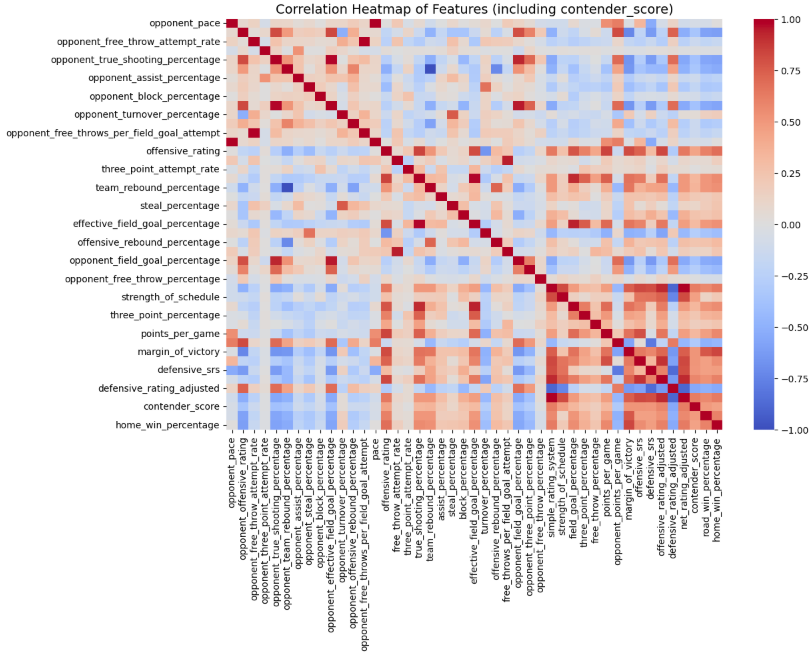
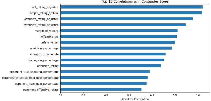
These correlation charts point out a few things:
Efficiencies: Net Rtg. and SRS showed strongest positive correlation
Road Win Percentage: It’s important that teams show they can win in tough environments
Strength of Schedule: Contenders face tough schedules that prepare them for March
Opponent TS%, eFG%, FG%, and O. Rtg.: Contenders are able to disrupt on defense and force their opponents into less efficient scoring opportunities
Regression Models
Which ML method works best on our dataset? For this, I didn’t just train a single model. Instead, I ran a model bake-off: a wide set of regression algorithms ranging from simple linear models to tree ensembles and gradient boosting. Each model was wrapped in the same preprocessing pipeline (imputation + scaling), so the comparison was fair.
The models I use include:
Baseline: a simple “predict the median” regressor as a sanity check.
Linear models: plain Linear Regression, Ridge, Lasso, and ElasticNet.
Distance- and kernel-based models: K-Nearest Neighbors (KNN) and Support Vector Regression (SVR).
Tree ensembles: Random Forest, ExtraTrees, and Gradient Boosting.
Modern gradient methods: HistGradientBoosting and XGBoost.
For each model, I evaluated two metrics:
R² (Coefficient of Determination) — Measures how much of the variation in the target (Contender Score) the model explains. Higher is better, with 1.0 = perfect prediction and 0 = no better than guessing the mean.
MAE (Mean Absolute Error) — The average size of the prediction errors, in the same units as the target. Lower is better. For example, an MAE of 4 means the model’s predictions are off by about 4 Contender Score points on average.
# ---------------------------
# Imports
# ---------------------------
from sklearn.dummy import DummyRegressor
from sklearn.linear_model import LinearRegression, Ridge, Lasso, ElasticNet
from sklearn.ensemble import RandomForestRegressor, ExtraTreesRegressor, GradientBoostingRegressor, HistGradientBoostingRegressor
from sklearn.svm import SVR
from sklearn.neighbors import KNeighborsRegressor
from sklearn.metrics import r2_score, mean_absolute_error
import pandas as pd
import numpy as np

try:
    from xgboost import XGBRegressor
    HAS_XGB = True
except Exception:
    HAS_XGB = False

# ---------------------------
# Define models
# ---------------------------
models = {
    "Baseline (Median)": DummyRegressor(strategy="median"),
    "LinearRegression": LinearRegression(),
    "Ridge": Ridge(alpha=5.0, random_state=42),
    "Lasso": Lasso(alpha=0.001, random_state=42, max_iter=20000),
    "ElasticNet": ElasticNet(alpha=0.05, l1_ratio=0.5, random_state=42, max_iter=20000),
    "KNN (k=7)": KNeighborsRegressor(n_neighbors=7, weights="distance"),
    "SVR (RBF)": SVR(C=5.0, epsilon=0.5, kernel="rbf"),
    "RandomForest": RandomForestRegressor(n_estimators=1000, max_depth=None, random_state=42, n_jobs=-1),
    "ExtraTrees": ExtraTreesRegressor(n_estimators=1000, random_state=42, n_jobs=-1),
    "GradientBoosting": GradientBoostingRegressor(random_state=42),
    "HistGradientBoosting": HistGradientBoostingRegressor(random_state=42),
}
if HAS_XGB:
    models["XGBRegressor"] = XGBRegressor(
        n_estimators=1200,
        learning_rate=0.05,
        max_depth=6,
        subsample=0.9,
        colsample_bytree=0.8,
        reg_lambda=1.0,
        random_state=42,
        n_jobs=-1,
        tree_method="hist",
    )

# ---------------------------
# Helper function to evaluate a regressor inside preprocessing pipeline
# ---------------------------
def evaluate_model(name, reg, preprocessor, X_train, y_train, X_test, y_test):
    pipe = Pipeline([("pre", preprocessor), ("reg", reg)])
    pipe.fit(X_train, y_train)
    preds = pipe.predict(X_test)
    return {
        "model": name,
        "R2": r2_score(y_test, preds),
        "MAE": mean_absolute_error(y_test, preds),
        "pipeline": pipe,
    }

# ---------------------------
# Run all models & collect results
# ---------------------------
results = []
for name, reg in models.items():
    try:
        res = evaluate_model(name, reg, pre, X_train, y_train, X_test, y_test)
        results.append(res)
        print(f"{name:>20}  |  R²: {res['R2']:.3f}  |  MAE: {res['MAE']:.3f}")
    except Exception as e:
        print(f"{name:>20}  |  ERROR: {e}")

# ---------------------------
# Leaderboard
# ---------------------------
leaderboard = (
    pd.DataFrame([{k: v for k, v in r.items() if k != "pipeline"} for r in results])
    .sort_values(["R2", "MAE"], ascending=[False, True])
    .reset_index(drop=True)
)
print("\nModel Leaderboard (higher R², lower MAE is better):")
print(leaderboard[["model", "R2", "MAE"]])

# Optionally grab the best fitted pipeline:
best_idx = leaderboard["R2"].idxmax()
best_name = leaderboard.loc[best_idx, "model"]
best_pipe = [r["pipeline"] for r in results if r["model"] == best_name][0]
print(f"\nBest model: {best_name}")| Model | R² | MAE |
|---|---|---|
| GradientBoosting | 0.767 | 4.465 |
| RandomForest | 0.755 | 4.634 |
| ExtraTrees | 0.753 | 4.710 |
| XGBRegressor | 0.747 | 4.749 |
| HistGradientBoosting | 0.731 | 4.917 |
| KNN (k = 7) | 0.671 | 5.312 |
| SVR (RBF) | 0.639 | 4.989 |
| Lasso | 0.463 | 9.073 |
| LinearRegression | 0.461 | 9.088 |
| Ridge | 0.461 | 9.132 |
| ElasticNet | 0.452 | 9.221 |
| Baseline (Median) | -0.188 | 7.600 |
GradientBoosting (R² = 0.77, MAE ≈ 4.5) came out on top, balancing strong predictive power with relatively low error.
Feature Importances
Next, I wanted to see which statistics the model relied on the most when predicting a team’s Contender Score. By extracting the feature importances from the best-performing model, we can identify the stats that consistently separate true contenders from everyone else.
<style>
import pandas as pd

importances = pd.Series(model.feature_importances_, index=X.columns).sort_values(ascending=False)
importances.head(10).plot(kind="barh")
plt.title("Top 10 Features by Importance")
plt.show()
</style>| Feature | Importance |
|---|---|
net_rating_adjusted |
0.509060 |
simple_rating_system |
0.111872 |
road_win_percentage |
0.065917 |
home_win_percentage |
0.045770 |
margin_of_victory |
0.011484 |
opponent_free_throw_percentage |
0.010957 |
three_point_percentage |
0.010426 |
opponent_three_point_percentage |
0.009833 |
strength_of_schedule |
0.009164 |
opponent_steal_percentage |
0.009055 |
assist_percentage |
0.008437 |
opponent_assist_percentage |
0.008384 |
opponent_block_percentage |
0.008328 |
defensive_rating_adjusted |
0.008100 |
defensive_srs |
0.007704 |
What stands out:
Adjusted Net Rating (0.51) dominates — this combined offensive/defensive margin is by far the strongest single predictor of contender status.
Simple Rating System (0.11) comes in second, reinforcing the value of all-around team strength.
Road (0.066) and Home (0.046) Win Percentages still appear prominently. These can be a little leaky if tournament games are included, but they capture consistency across environments.
Margin of Victory and Defensive metrics — margin of victory (0.011), adjusted defensive rating (0.008), and defensive SRS (0.008) all show up, highlighting that elite defenses continue to matter.
Shooting efficiency matters — both a team’s own 3PT% (0.010) and their opponent’s 3PT% (0.010) play important roles, reminding us how much the perimeter game can swing outcomes.
Supporting cast features — opponent FT% (0.011), opponent steals, blocks, and assists (all around 0.008–0.009), along with assist percentage (0.008), provide smaller but meaningful contributions. These capture discipline, ball movement, and defensive disruption.
Strength of Schedule (0.009) remains in the mix, showing that teams tested against tougher competition are more likely to survive March.
Wrapping Up
The GradientBoosting model (and other ensemble methods) can predict Contender Scores within about 3–5 points on average. That’s impressively accurate given the chaos of March Madness. Of course, there will always be outliers — 2014 UConn making a surprise run from a 7-seed or 2023 FAU storming to the Final Four — but even those Cinderella stories stand out precisely because they’re rare exceptions to the rule.
When you zoom out across thousands of team-seasons, the data paints a clear, consistent profile of what true contenders look like:
Efficiency rules — Adjusted Net Rating absolutely dominates the model. Teams that outscore their opponents by wide margins on a per-possession basis are almost always in the title conversation.
Consistency counts — Home and road win percentages rise to the top of the importance list. Contenders don’t just rack up wins at home; they prove they can survive in hostile environments.
Defense still wins — Opponent shooting metrics (eFG%, 3P%, FT%) and defensive efficiency underline that limiting opponents is a defining trait of champions. You can’t just outscore everyone — stops matter.
Strength of Schedule matters — Contenders are forged against tough competition. Teams that cruise through weak schedules may look good on paper, but the model recognizes that they’re less prepared for the gauntlet of March.
Supporting stats add nuance — Features like assist %, turnover/steal rates, and margin of victory don’t carry the same weight as net rating, but they sharpen the edges of the contender profile by capturing discipline, ball movement, and the ability to execute under pressure.
Put simply: the numbers confirm what coaches and fans have long believed. True contenders are efficient, balanced, resilient, and battle-tested. While upsets will always capture headlines, the data shows that championships are built on fundamentals that consistently show up in the stats.
Do you think that your team has what it takes? Make sure to keep an eye out for these key indicators the next time you are watching your favorite team to tell if they might be able to truly contend for a National Championship!